Rev 2 12/7/2023
Stephen Connell KC1SVE
There are matching tools available to calculate and design an impedance matching circuit in moments. One example is provided by Analog devices Inc.’s online design center tool RF Impedance Matching Calculator.
Another online tool that is helpful is the Telestrian Interactive Smith Chart. It doesn’t do the design for you, but it shows you the effects of adding matching components. You can plug in the load impedance, set the series matching components to a short circuit and the parallel components to an open and it shows you where your impedance lies on the Smith chart. You can then add your matching components to view how the impedance point moves on the chart.
Link: http://cgi.www.telestrian.co.uk/cgi-bin/www.telestrian.co.uk/smiths.pl
I was curious though, what’s the magic behind these tools? Sometimes it helps to know, for when things go awry. This section describes the procedure that I worked out should I ever have to “do it myself”.
My approach here is to try to limit this discussion to what MUST be done and WHY I am doing it. I’m trying to keep it simple with enough information to recall what I was thinking at the time, so I can do it again when I want to.
A basic understanding of resistance, reactance, (resistors, inductors and capacitors) and the Smith chart is required. For learning about the Smith chart, I highly recommend Basics of the Smith Chart, Alan Wolke’s (W2AEW) online presentation. This is the first time I’ve actually used a Smith Chart for a practical application so, I’m certainly not an expert. It might be helpful though to follow me here to see how I finally got it to work for me.
Objective
I have a Radio Transceiver designed to operate with a 50-ohm antenna (load) impedance. I want to match my antenna (load) impedance to the Radio (source) impedance. Why? The match is needed so that the Transmit signal does not reflect back from the load to the source AND when I receive a signal, I don’t want the signal to reflect back up the antenna. Reflections are bad because they return the RF signal to the radio (or antenna) reducing the power for the antenna to radiate (or the radio to receive). In the transmit case it could also damage the radio if the reflected power exceeds the radio’s ability to dissipate the energy. If we match the source and load impedances, we won’t have reflections, so all of the power will be radiated (or received). When matched(equal) their ratio will be 1:1 of course. This is our goal; it is referred to as a Voltage Standing Wave Ratio (VSWR). We want this to be 1.
Objective – > VSWR = 1.0
Antenna Impedance
The antenna has impedance to signal flow. The impedance is due to its resistance, inductance and capacitance. These are the three components that we need to know about to describe what is impeding the signal flow. The resistance (R) is kept very low by using conductors that are large enough to avoid dissipating heat energy. Resistance is NOT dependent on frequency. The inductance and capacitance also impede the signal flow. This impedance IS frequency dependent, it’s called reactance, designated by X. Reactance depends on the geometry of the antenna, where you are connected to it, and how it sits in the electric and magnetic fields that it generates and that exist around it (from things like the earth and other conductors). The geometries of the conductors effectively create inductors and capacitors, just like the components we can buy. Because their impedance is frequency dependent, as we transmit or try to receive signals of different frequencies this impedance changes as well. So, if we want the antenna to work well (limited signal loss due to reflections) we need to design matching circuits for the frequency ranges we plan on using. Because of this frequency dependence, we need to measure and track this impedance separately from resistance. Since frequency is the common factor for both inductor and capacitor impedance, we can combine them into a single reactance term (X). The resulting equation to describe impedance is:
Impedance equation Z = R + jX Where R (resistance) is NOT frequency dependent and X (reactance) IS frequency dependent.
Impedance (Z) and Admittance (Y = 1/Z)
So, we have impedance that can be described by physical passive components (resistors, inductors and capacitors). What is Admittance and why do we need it? Admittance is described by the equation G +jB, where G is the conductance (1/R – frequency independent) and B is the susceptance (1/X- frequency dependent). Do we have passive components that can conduct? And, what is susceptance? It turns out that when we add any of the three passive components in parallel to the load, instead of in series, the circuit will conduct more current and it is more susceptible to passing the frequency dependent current (AC). We need to know about admittance because it gives us a way to describe what happens when we add components in parallel to the load, and even better a way to directly plot these changes on a Smith chart. In short, it depends on how the component is placed in the circuit. If it’s added in series, it will increase the impedance. If it’s added in parallel it will decrease the impedance by the inverse of its value. Therefore, admittance is defined by Y = 1/Z. Admittance will make it possible to graphically move on the Smith chart when we’re adding parallel components, that’s why we need it.
The Smith Chart
The basic Smith chart is a plot of impedances with constant resistance (R) circles and constant reactance (X) arcs, both plotted from 0 to infinity. It’s a chart that we can plot our measured impedance onto. The normalized resistance value of 1 (reactance = 0) is at the center of the chart. By normalized, it means we divide all of our impedances by the system (or source) impedance. So, in our case the center normalized value represents a perfect 50-ohm resistance with 0-ohms reactance. Once normalized any measured impedance can be plotted on the chart. The center point (1) is going to be the target location that we want to match the load impedance to. This is where the source and load impedances are equal to each other; the VSWR is 1.
To move our load impedance to the center point we will be adding only inductors and capacitors, no resistors. We don’t want to dissipate power as heat by adding resistors, the inductors and capacitors will store and return the power to the circuit. As we add inductors and capacitors, we will be changing the reactance, the resistance does not change; it remains constant. This means we will be moving along the circles only (constant resistance circles). How can we get to the center if we are stuck on circles?
This is why we need to know about admittance. If we draw admittance lines (constant conductance circles and constant susceptance arcs) we see that we get another set of lines, except that 0 and infinity are swapped (everything is inverted). Combined charts are available, that already have both impedance and admittance lines plotted. It turns out that the plots are identical, except that they are rotated 180 degrees from each other. This makes perfect sense because the right side of the impedance chart is 0-ohms and the left is infinite ohms, and we know that Y = 1/Z. So, if you flip one around 180 degrees, you’ve got the other.
We need the admittance chart to add parallel components. This will allow us to add inductors and capacitors in parallel. In this case, we will be changing the susceptance (1/X reactance) as we move along constant conductance circles (1/R in this case). If you don’t have a combined Smith chart no worries, it can be done with just the impedance lines plotted, which is what I will describe here. Because they are the same plots, just rotated by 180 degrees, we can just replot impedance points to a rotated 180-degree location and then view the impedance chart as though it’s an admittance chart. You can then go back and forth using one chart for parallel components and series components simply by doing this. It’s not as difficult as it sounds. The procedure below will show you how.
Circuit Requirements
- Design a circuit using inductors and capacitors to achieve the impedance match.
- To cover all potential load impedances will require parallel and series components that will be arranged in one of two possible topologies.
Z2series topo Z2parallel topo
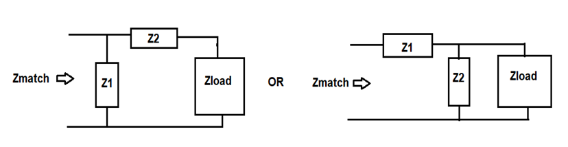
- Determine if Z1 and Z2 are inductors or capacitors.
- Determine the values of the components.
Procedure
- Determine the Load impedance (Zload) at the Frequency (f) that you wish to match. I like using an inexpensive vector network analyzer, such as the nanoVNA for this.
Example: Impedance: ZL = 37 + j16, Frequency: f = 21.25MHz
- Normalize Zload: We are working in a 50-ohm system, so we divide the values by 50 to normalize.
Example: Zload = 37/50 + j16/50 = .74 + j.32
- Use the impedance Smith chart. Our goal is to plot our impedance as it is and then to add our matching components to move that impedance to the middle of the chart (1). As noted previously, It’s where the VSWR = 1 (50-ohm match). We are only adding inductors and capacitors, no resistors. This means that we will only be changing reactance, so resistance will stay constant. Therefore, our movement is confined to the constant resistance circle that we are on.
How can we get to the center (1) if we are stuck on a constant resistance circle? We can’t, so we add the admittance chart. We’ll get another set of circles and arcs that intersect the impedance circles and arcs. These circles will be constant conductance circles. You can use a combined Smith chart that shows both if you have one. For this procedure, I’ll proceed with the simple impedance only smith chart.
- Continuing with the Impedance only chart, we need to add an important constant conductance = 1 circle. Let’s add that circle (see below) and lets also highlight the constant resistance = 1 circle.
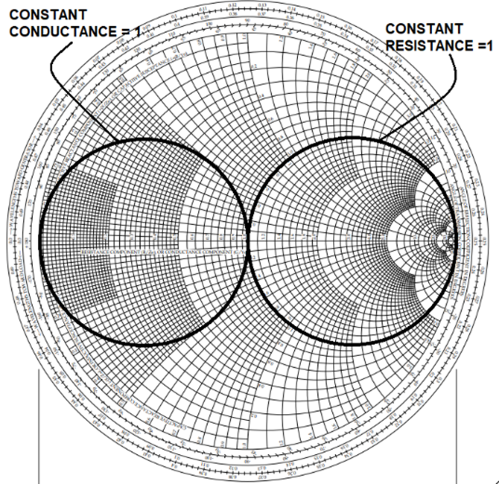
We need these two circles for two reasons: 1. They will define which of the two topographies we will use (Z2series or Z2 parallel). 2. They will identify all points on the chart where the resistance and conductance are equal to our target of 1. (50 ohms). Since we can only move along circles, and we only want to add 2 components, when we add our first component, we want to move our impedance to a point on one of these circles. Then, we will only need to add one more component to move along one of these circles to the get to the center of the chart.
Plot the normalized Zload (.74_j.32) on the chart.
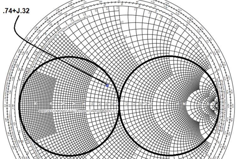
The .74 resistance is read along the center horizontal. The .32 reactance is read from the perimeter, where the arcs terminate.
- Eventually, we want to move this impedance to the center point of the chart, but the first component we add must get us to a point on one of these two circles. We know that adding inductors and capacitors moves us along constant resistance or constant conductance circles. Looking at our plotted impedance, we see that we can move along a constant resistance circle to get to the constant conductance circle = 1. Let’s do that.
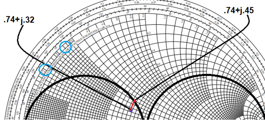
We moved along a constant resistance circle from .74+j.32 to .74+j.45, therefore, we have added .13 reactance in series with the load. This means that we must use the Z2series topology. Notice that for any impedance we start with that lies inside the constant conductance circle we MUST use the Z2series topology because the only circles that intersect the conductance =1 circle are constant resistance circles. The opposite holds true for the constant resistance circle. If we are inside the constant resistance circle, we MUST use the Z2parallel topology. What if we are outside these two circles? In that case, you get a choice, either topology can be made to work.
What else did we already determine? We added .13 reactance. Anytime we ADD reactance we are adding an inductor. So, the series componentis an inductor. Notice that we could have moved in a negative j direction and reached the bottom edge of the circle. In this case we would be subtracting reactance. Anytime we SUBTRACT reactance we are adding a capacitor. It’s your choice. Back to our inductor, we also know the value of the inductor by the amount of reactance (.13) that we added. We’ll figure that out at later.
- We are now on the admittance circle =1, and it goes right thru the center point (1). This is good, we can move along this circle with one more component to get to the center. When we move along a constant conductance circle, we are adding a component in parallel.
- If you have a combined Admittance/Impedance Smith chart: You can now move toward the center along this circle, noting that you will move -j.63. Moving in a negative j direction is subtracting susceptance. Thismeans that this component is a capacitor. And, since this is a susceptance value (B=1/X) we need to invert it to find the reactance X= 1/.63 = 1.59.
If you only have an impedance Smith chart: Notice that if we move along the constant conductance = 1 circle there aren’t any arcs that go to the perimeter where we can read the change in reactance. However, since we know that the admittance chart is the same as the impedance chart except that it is rotated 180 degrees, we can replot our impedance to a location 180 degrees around the chart. We will then use the impedance Smith chart (with labeled arcs) as though it is an admittance Smith chart. We will have to remember though that we effectively rotated our chart 180 degrees. Up is now down and down is up. So, moving in the negative j direction is really moving positive and vice versa. We will have to remember this since the + or – sign of our direction movement determines if it’s a capacitor or an inductor that we adding.
To do this: Replot the impedance 180 degrees around the chart: Draw a circle, centered at the center of the chart with the radius set to the impedance. Next draw a line from the plotted impedance thru the center to the opposite side of the same circle.
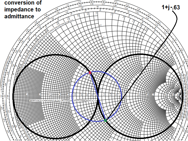
From this point we can now use the constant resistance=1 circle to get to the center point. We now have j values at the perimeter that we can use. We see that we are going to have to move +j.6 to get to the center. But remember, the chart has been spun 180 degrees. Therefore, we are really moving -j.63 not +j.63. So, we are adding a capacitor (- movement) not an inductor (+ movement). Again, we are working in the admittance domain, just using the impedance chart so we can read values from the perimeter. Therefore, the component is to be added in parallel and, we must invert the susceptance value (B) to find the reactance (X=1/B) of the component we are adding. Therefore X = 1/.63 =1.59.
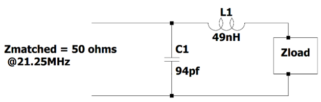
- Knowing the impedance, we can calculate the values for the Inductor and Capacitor.
ZL = .13*50 = 6.5, 6.5 = 2**f*L, L = 49nH
ZC = 1.59*50 = 79.5, 79.5 = 1/(2**f*C), C = 94pf
- The components we select must also be capable of handling the currents and voltages that will be present. You must meet the maximum voltage spec for the capacitor and the maximum current spec for the inductor. If you don’t the components could be damaged, or even cause a fire hazard. For this example, our Transmitter can deliver 100 watts of power. Power is calculated using RMS values, so the RMS voltages and currents can be calculated by these formulas; P=I2*R and P=I*V, if we know the resistance. The Transmitter is designed to operate in a 50-ohm system. Using the equations, we calculate; Vrms=70.7 volts, Irms=1.414 amps. The component ratings are in peak voltages, so we need to convert the rms values to peak values. Divide by .707 to get the peak values. The peak voltages and currents are then V=100 volts, and I = 2 amps. We could see 2X’s these values due to reflections when we are not matched. That gets us up to V=200V and I=4A. For capacitors the rule of thumb is to use a capacitor with a voltage rating of 2X the voltage, so a minimum capacitor rating of 400V would suffice. It’s easy to find inexpensive capacitors rated to 500V and into the thousands. I like to wind my own inductors, so I would use magnet wire that can handle at least the 4A. #22 wire is rated to 7A for chassis wiring. This is a non-bundled spec. Depending on the inductance our windings could become fairly dense, so take care for large values of inductance. I would expect #22 to be fine for most inductors being designed for this application. Anyway, I have been using #20 wire rated to 11A chassis and #18 wire rated to 16A chassis without any issues.